5.1.1 Tikhonov regularisation method
by A. Matulis and Z. Kancleris
Treating the integral equation given in the Introduction numerically one has to perform the discretisation which leads to the system of linear equations. In the matrix notation it can be represented as follows:
|
|

Here  1 is
the transient represented at some (usually equidistant) time intervals,
1 is
the transient represented at some (usually equidistant) time intervals,
 2 is
the exponential kernel matrix
2 is
the exponential kernel matrix  3 and
3 and
 4 is
a vector representing the spectrum at some given frequency points which we are
looking for.
4 is
a vector representing the spectrum at some given frequency points which we are
looking for.
The linear system can not be solved directly for any 5. It
confirms the diagonalization of the kernel matrix. For instance, more than 80%
of the eigenvalues do not exceed in magnitude the computer accuracy if the
matrix 100 x 100 is considered. Changing the above matrix equation into the
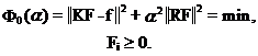
minimization problem
|
|

we arrive at the ill-conditioned problem that can not be treated without some additional means, because usually there are many possible solutions of problem (2) satisfying it within the experimental transient errors. In order to treat the above problem properly we added some additional information by means of inequality constraints (it is known that all spectrum components should be positive), and included the Tikhonov regularisation. In a such way we arrived to the following minimisation problem
|
|
We used the regularisation matrix
 6
which action on the spectrum corresponds to the calculating of the second
derivative. The magnitude of the regularisation parameter
6
which action on the spectrum corresponds to the calculating of the second
derivative. The magnitude of the regularisation parameter  7
characterises the influence of the regularisation on the spectrum. This
parameter plays the same role as a filter bandwidth when smoothing noisy data.
It can not be chosen to small due to the above mentioned ill-conditions of the
problem. Besides, in that case the artefacts in spectrum starts to appear. It is
also evident that it can not be chosen too large because in that case the
solution will be shifted far away from the expected solution of our initial
problem (1).
7
characterises the influence of the regularisation on the spectrum. This
parameter plays the same role as a filter bandwidth when smoothing noisy data.
It can not be chosen to small due to the above mentioned ill-conditions of the
problem. Besides, in that case the artefacts in spectrum starts to appear. It is
also evident that it can not be chosen too large because in that case the
solution will be shifted far away from the expected solution of our initial
problem (1).
The algorithm
Two algorithms [1,2] are mainly used for treating the Fredholm equations of the first kind. We employed the Provencher's method [1] since it seems to be more flexible. In particular case of equation (3,4) the above method can be essentially simplified, and reduced to the application of twofold singular value decomposition (SVD) [3]:
|
(7) |
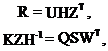
where  8 and
8 and
 9 are
the diagonal matrixes while
9 are
the diagonal matrixes while  10,
10,
 11,
11,
 12
and
12
and  13
are the orthogonal ones. Here superscript T stands for denoting the matrix
transpose. Making the following change in the variables
13
are the orthogonal ones. Here superscript T stands for denoting the matrix
transpose. Making the following change in the variables
|
|

and taking into account (6) and (7) we arrive at the final minimization problem with the inequality constraints
|
(10) |

Here the following notations are used
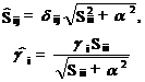
(11)
(12)
|
|

and
The obtained minimization problem was treated using Least distance programming method (LDP) [4].
The main advantage of the above technique is that the most computer time consuming procedures (SVD) are carried out only once for a given transient, and then the solutions for various regularisation strengths can be easily obtained applying rather fast LDP procedure.
Results and discussion
In order to establish the application of the above technique in the case of a wide spectrum we performed numerical calculations with the artificially simulated transients. They were composed of a single Gaussian spectrum component
|
|

with the following parameters  14,
14,
 15.
The transients consisting of 1000 equally spaced points were used with some
Gaussian noise added. Typical noise to signal ratio (NSR) at t=0 was in the
range 10-2...10-3. Spectrum has been calculated for 100
equidistant points in the range 0...2 Hz.
15.
The transients consisting of 1000 equally spaced points were used with some
Gaussian noise added. Typical noise to signal ratio (NSR) at t=0 was in the
range 10-2...10-3. Spectrum has been calculated for 100
equidistant points in the range 0...2 Hz.
The main output of the calculations was the several average functions which we hoped could be sensitive to the regularisation parameter choice. The following functions were examined:
(i) declination of the solution of minimization problem (9,10) from the exact minimum
|
|

that is usually caused by the inequality constraints;
(ii) standard deviation of a residual, that is defined as the difference between the initial transient and its fit
|
|

and (iii) some special function
|
|
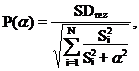
that was introduced by Provencher [1] as a
suitable criterion for 16
choice. Here  17 is
the number of points in the calculated spectrum and the sum in the denominator
indicates so called the "degrees of freedom" of considered minimization
problem.
17 is
the number of points in the calculated spectrum and the sum in the denominator
indicates so called the "degrees of freedom" of considered minimization
problem.
References
1. S.W. Provencher, Comp. Physics Communications, V. 27, p. 213, 1982.
2. J. Weese, Comp. Physics Communications, V. 69, p. 99, 1992.
3. W.H. Press, S.A. Teukolsky, W.T. Veterling, B.P.Flannery, Numerical recipes in C (Cambridge, University Press, 1995).
4. C.L. Lawson, R.J.Hanson, Solving least squares problems (Philadelphia, SIAM, 1995)